Affymetrix Facility Documentation


		Affy Facility Docs Home

	Running Chips

		Pricing Sample Submission

	SBEAMS

		Download Data Annotate Samples GetExpression Get Affy Intensity

	Analize Data

		Analysis Pipeline MEV

	Affy Help Pages

		Affy Core Help SBEAMS Help Pages Analysis Help Pages Tutorials and Presentations

	Other Resources

		Affymetrix Home Page

R vs. GCOS MAS5 Comparison

Comparison of GCOS/MAS5.0 Output and Bioconductor/affy/mas5 Output. Evaluated on Mouse 430 2.0, HG-133 Plus 2.0 and YG_S98 chips.

Getting GCOS/MAS5 data
In GCOS, double-click names of .CHP files desired. Data is displayed in tabular format, choose File->Save to save it out.

Getting R/Bioconductor/affy/mas5 data
Create a list file with a few chips of each chip type. The first line is the chip name, second line is always blank and starting with the third line are the CEL file names. Both the directory under Affymetrix/core/probe_data and the actual CEL file name must be included.

LPS_0_120.list
Mouse430_2 200406/20040621_01_LPS2-0.CEL 200406/20040622_01_LPS3-0.CEL 200406/20040621_06_LPS2-120.CEL 200406/20040622_06_LPS3-120.CEL

YG_S98-test.list
YG_S98 200409/20040920_01_G848I.CEL 200409/20040920_02_G848II.CEL 200409/20040922_03_G848III.CEL 200408/20040831_05_G984II.CEL 200409/20040916_02_G984II.CEL 200408/20040831_06_G984III.CEL

hgu133plus2-test.list
/net/arrays/Affymetrix/core/probe_data/200404/20040421_01_LN_1.CEL /net/arrays/Affymetrix/core/probe_data/200404/20040421_02_LN_2.CEL /net/arrays/Affymetrix/core/probe_data/200404/20040421_03_C4-2_2.CEL

Bioconductor Steps

For each chip type, use R/Bioconductor

R can be downloaded from

(http://www.r-project.org)

2) Bioconductor packages can be installed by running within R:


source("http://www.bioconductor.org/getBioC.R")
getBioC()

3) Then run in R

file.table.name <- “<list file name>”
output.file.name <- “<list name>.txt”
switch(.Platform$OS.type, unix = .libPaths("/net/arrays/Affymetrix/bioconductor/library/"),"windows")
require(affy)
ft <- read.table(file=file.table.name,sep="\t",blank.lines.skip=FALSE)
ft.character <- c(as.vector(ft$V1))
setwd(switch(.Platform$OS.type, windows = "Z:/Affymetrix/core/probe_data","/net/arrays/Affymetrix/core/probe_data"))
data <- read.affybatch( filenames = c(ft.character[ 3:length(ft.character) ]) )
eset <- mas5(data,sc=250)
PACalls <- mas5calls(data)

Matrix <- exprs(eset)
output <- cbind(row.names(Matrix),Matrix,se.exprs(PACalls))
write.table(output,file=output.file.name,sep="\t",row.names=FALSE)

Comparison of Signal Values

Signal values between R and GCOS show Pearson correlation of approximately 1, and slope very near 1.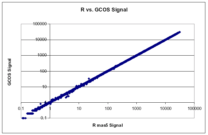

Open Link

R vs GCOS Excel Data

Comparison of Detection p-values
Detection p-values show a Pearson correlation near 1, however there are large differences in the low p-values that are masked by good correlation of large p-values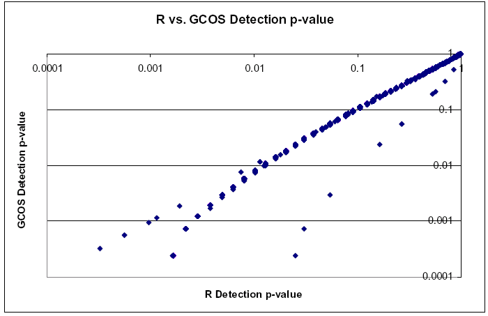

Comparison of Detection Calls

Fortunately, differences in Detection p-values are not of great concern since it is the Detection Call that is actually used. For detection calls, Affy currently says p < 0.05 is P(present), 0.05 < p < 0.065 is M(marginal) and p > 0.065 is A(absent). Using these cutoffs, 4 Mouse 430 2.0 and 3 Hg-U133 Plus 2.0 gave a total of only 45/344429(0.013% difference) calls incorrect due to differences between R and GCOS. The reason there are any discrepancies at all is that while Affymetrix has disclosed their method for making detection calls, implementing the method as they describe it does not reproduce the results GCOS produces.